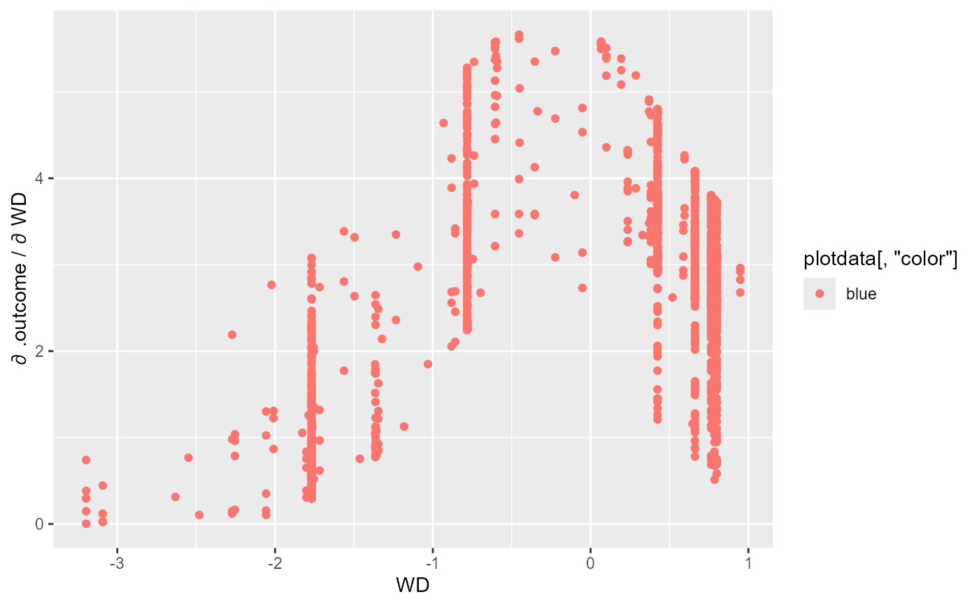
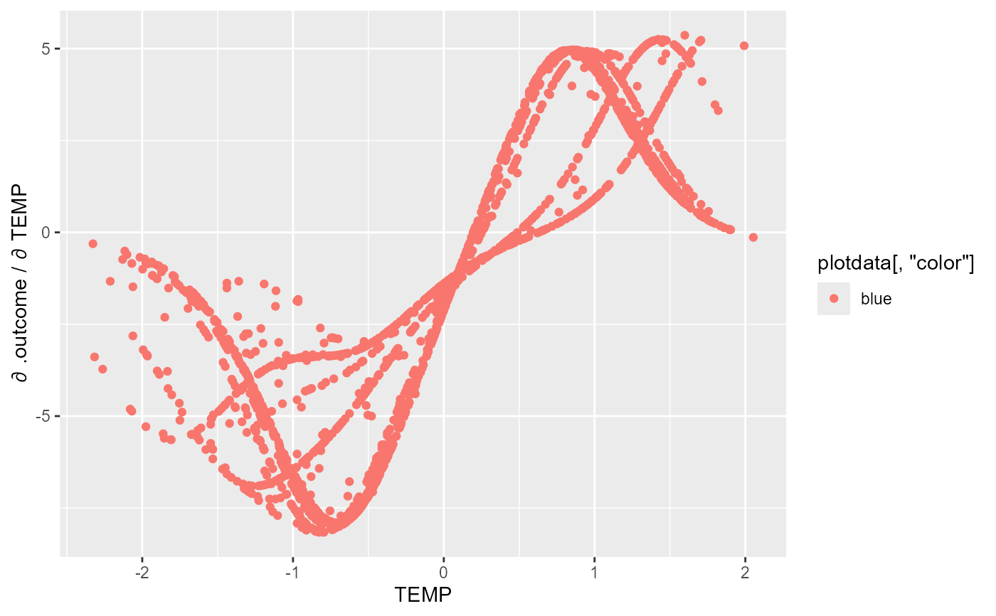
Plot of sensitivities of the neural network output respect to the inputs
Usage
SensDotPlot(
  object,
  fdata = NULL,
  input_vars = "all",
  output_vars = "all",
  smooth = FALSE,
  nspline = NULL,
  color = NULL,
  grid = FALSE,
  ...
)
Arguments
- object
fitted neural network model or
arraycontaining the raw sensitivities from the functionSensAnalysisMLP- fdata
data.framecontaining the data to evaluate the sensitivity of the model.- input_vars
character vectorwith the variables to create the scatter plot. If"all", then scatter plots are created for all the input variables infdata.- output_vars
character vectorwith the variables to create the scatter plot. If"all", then scatter plots are created for all the output variables infdata.- smooth
logicalifTRUE,geom_smoothplots are added to each variable plot- nspline
integerifsmoothis TRUE, this determine the degree of the spline used to performgeom_smooth. Ifnsplineis NULL, the square root of the length of the data is used as degrees of the spline.- color
characterspecifying the name of anumericvariable offdatato color the scatter plot.- grid
logical. IfTRUE, plots created are show together usingarrangeGrob- ...
further arguments that should be passed to
SensAnalysisMLPfunction
Value
list of geom_point plots for the inputs variables representing the
sensitivity of each output respect to the inputs
Examples
## Load data -------------------------------------------------------------------
data("DAILY_DEMAND_TR")
fdata <- DAILY_DEMAND_TR
## Parameters of the NNET ------------------------------------------------------
hidden_neurons <- 5
iters <- 250
decay <- 0.1

################################################################################
#########################  REGRESSION NNET #####################################
################################################################################
## Regression dataframe --------------------------------------------------------
# Scale the data
fdata.Reg.tr <- fdata[,2:ncol(fdata)]
fdata.Reg.tr[,3] <- fdata.Reg.tr[,3]/10
fdata.Reg.tr[,1] <- fdata.Reg.tr[,1]/1000

# Normalize the data for some models
preProc <- caret::preProcess(fdata.Reg.tr, method = c("center","scale"))
nntrData <- predict(preProc, fdata.Reg.tr)

#' ## TRAIN nnet NNET --------------------------------------------------------
# Create a formula to train NNET
form <- paste(names(fdata.Reg.tr)[2:ncol(fdata.Reg.tr)], collapse = " + ")
form <- formula(paste(names(fdata.Reg.tr)[1], form, sep = " ~ "))

set.seed(150)
nnetmod <- nnet::nnet(form,
                      data = nntrData,
                      linear.output = TRUE,
                      size = hidden_neurons,
                      decay = decay,
                      maxit = iters)
#> # weights:  21
#> initial  value 2487.870002
#> iter  10 value 1587.516208
#> iter  20 value 1349.706741
#> iter  30 value 1333.940734
#> iter  40 value 1329.097060
#> iter  50 value 1326.518168
#> iter  60 value 1323.148574
#> iter  70 value 1322.378769
#> iter  80 value 1322.018091
#> final  value 1321.996301
#> converged
# Try SensDotPlot
NeuralSens::SensDotPlot(nnetmod, fdata = nntrData)