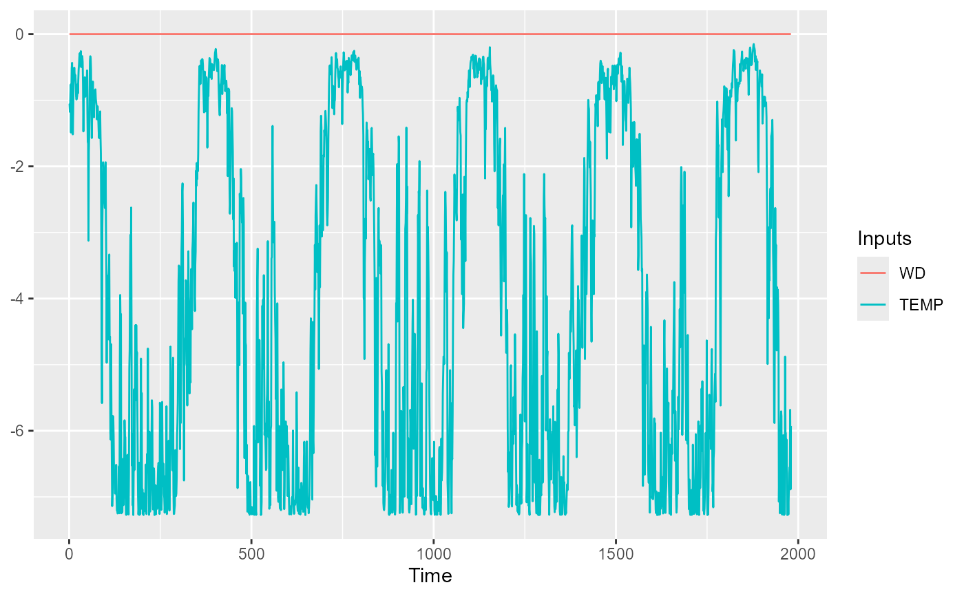
Sensitivity analysis plot over time of the data

Plot of sensitivity of the neural network output respect to the inputs over the time variable from the data provided

Usage

SensTimePlot(
  object,
  fdata = NULL,
  date.var = NULL,
  facet = FALSE,
  smooth = FALSE,
  nspline = NULL,
  ...
)

Arguments

object: fitted neural network model or array containing the raw sensitivities from the function SensAnalysisMLP
fdata: data.frame containing the data to evaluate the sensitivity of the model. Not needed if the raw sensitivities has been passed as object
date.var: Posixct vector with the date of each sample of fdata If NULL, the first variable with Posixct format of fdata is used as dates
facet: logical if TRUE, function facet_grid from ggplot2 is used
smooth: logical if TRUE, geom_smooth plots are added to each variable plot
nspline: integer if smooth is TRUE, this determine the degree of the spline used to perform geom_smooth. If nspline is NULL, the square root of the length of the timeseries is used as degrees of the spline.
...: further arguments that should be passed to SensAnalysisMLP function

Value

list of geom_line plots for the inputs variables representing the sensitivity of each output respect to the inputs over time

References

Pizarroso J, Portela J, Muñoz A (2022). NeuralSens: Sensitivity Analysis of Neural Networks. Journal of Statistical Software, 102(7), 1-36.

Examples

## Load data -------------------------------------------------------------------
data("DAILY_DEMAND_TR")
fdata <- DAILY_DEMAND_TR
fdata[,3] <- ifelse(as.data.frame(fdata)[,3] %in% c("SUN","SAT"), 0, 1)
## Parameters of the NNET ------------------------------------------------------
hidden_neurons <- 5
iters <- 250
decay <- 0.1

################################################################################
#########################  REGRESSION NNET #####################################
################################################################################
## Regression dataframe --------------------------------------------------------
# Scale the data
fdata.Reg.tr <- fdata[,2:ncol(fdata)]
fdata.Reg.tr[,3] <- fdata.Reg.tr[,3]/10
fdata.Reg.tr[,1] <- fdata.Reg.tr[,1]/1000

# Normalize the data for some models
preProc <- caret::preProcess(fdata.Reg.tr, method = c("center","scale"))
#> Warning: These variables have zero variances: WD
nntrData <- predict(preProc, fdata.Reg.tr)

#' ## TRAIN nnet NNET --------------------------------------------------------
# Create a formula to train NNET
form <- paste(names(fdata.Reg.tr)[2:ncol(fdata.Reg.tr)], collapse = " + ")
form <- formula(paste(names(fdata.Reg.tr)[1], form, sep = " ~ "))

set.seed(150)
nnetmod <- nnet::nnet(form,
                      data = nntrData,
                      linear.output = TRUE,
                      size = hidden_neurons,
                      decay = decay,
                      maxit = iters)
#> # weights:  21
#> initial  value 2518.847637 
#> iter  10 value 1980.676972
#> iter  20 value 1863.605952
#> iter  30 value 1714.408226
#> iter  40 value 1702.860135
#> iter  50 value 1697.085071
#> iter  60 value 1696.693269
#> iter  70 value 1696.690378
#> final  value 1696.690265 
#> converged
# Try SensTimePlot
NeuralSens::SensTimePlot(nnetmod, fdata = nntrData, date.var = NULL)
#> Warning: Use of `plotdata$value` is discouraged.
#> ℹ Use `value` instead.
#> Warning: Use of `plotdata$variable` is discouraged.
#> ℹ Use `variable` instead.
#> Warning: Use of `plotdata$variable` is discouraged.
#> ℹ Use `variable` instead.